Hello again :)

In part 2, we’re going to cover the tool I built to teach a battery when to store and sell back electricity to the grid, and test how well it would have done using historical electricity price data.

We’ll go through the different parts of the tool: a linear program (LP) that finds the optimal charge/discharge schedule given a 24-hour price forecast, the forecasting models that feed into the LP, a backtester that runs the results against real market data, and a Streamlit dashboard I built to make the experience more interactive.

But first… Quick recap:

Because electricity prices move a lot, batteries can exploit those price swings by charging when prices are cheap, and discharging when the price goes up in times of higher demand or grid stress.

The question “when should batteries charge and discharge?“ might sound trivial, but it isn’t, for a few reasons.

Decisions are coupled across time. Charging at 3am, for example, affects what you can do at 7am. At every hour of the day, each decision made on whether now is a good time to buy/sell electricity affects what is available for the rest of the day. You could discharge too aggressively into the morning peak hours, but that could leave you empty during the evening peak, which is usually the most expensive window of the day, all things considered.

We have to respect physical limits. Each charge/discharge cycle wears the battery out a bit, and that wear has a cost(the lifetime value of the battery reducing) and it can determine whether a given price spread is worth trading at all. There’s also a maximum amount of energy you can store(capacity measured in MWh), a maximum rate at which you can charge/discharge(power rating measured in MW), and you can’t discharge energy you haven’t got, obviously.

You don’t have tomorrow’s prices. Operators clear a charging schedule based on a forecast of electricity prices at each hour for the next day, which you can’t confirm until the day-ahead auction clears the following morning.

The first two constraints go into the optimizer, and the third is the forecasting problem, which informs the backtesting results, connecting it to the real world.

So, What Are We Solving? #

The optimizer needs to know what it’s trying to maximize, what physical rules it can’t break, and what it costs to use the battery to charge/discharge. This means:

For a single battery, over a 24-hour period, at what hours should the battery charge/discharge in order to maximize profit, also taking into account the cost of degradation?

Our objective function looks like this:

The degradation penalty ($C_{deg}$) applies to the total throughput n both directions, as opposed to just discharge. This is because every MWh that flows through the battery eats at a small amount of its usable life, so both $p_t^c$ and $p_t^d$ count against it.

And our objective function is subject to the following constraints:

• The energy in the battery next hour equals the energy in the battery this hour, plus whatever was charged(scaled by charging efficiency), minus whatever was discharged (divided by discharge efficiency to account for losses on the way out). This is called the SoC balance.

• We also force the battery back to its starting state at the end of the 24-hour window. Without it, the optimizer would discharge everything at the end of the time period because it has no knowledge of tomorrow. Adding in this constraint makes sure that each day’s solution is repeatable and consistent. This is called the Terminal SOC.

• Charge and discharge power both have to be non-negative and bounded by the battery’s maximum power rating P.

• State of charge is also bounded between empty and the battery’s maximum capacity E.

• The round-trip efficiency is split symmetrically. For example, if the round-trip efficiency is 90%, both sides get √0.9, which is roughly equal to 0.949. Real batteries have asymmetric losses, so this makes modelling more convenient. It’s also the standard assumption when you only have a single round-trip figure to work with.

• And optionally, to prevent the solver from trying to charge and discharge simultaneously, we can add a binary variable z_t that forces the battery to commit to one mode per timestep. In pure LP, nothing prevents the solver from trying to charge and discharge at the same time, but with perfect round-trip efficiency, this would be equivalent to doing nothing, so the result isn’t changed either way. This would convert our LP problem into a Mixed Integer Linear Program(MILP), and I set this to be an opt-in on the dashboard for transparency.

The Forecasting Pipeline #

Training the model is the straightforward part. The harder problem is trying to make predictions the way an operator would need them; the day before, using only what was known at that time.

We need 24-hourly forecasts for tomorrow, ready before the day-ahead market closes. Every feature used to generate those predictions, must come from information that was available before the target window that could implicitly encode tomorrow’s prices.

There are two common ways to violate this rule:

• Computing rolling statistics on the full time series before splitting to get your train/test sets. The rolling window for early rows will look forward past the split boundary if we do this.
• Randomly splitting to get the train/test sets instead of chronologically splitting. Doing this doesn’t make sense because the test set will definitely end up containing data from before the training’s set time range.

Doing either of these would give you suspiciously clean metrics, but if you get terrible results in deployment, you can start checking from here.

Model 1 - Naive Lag-24 #

This model makes prediction based on the assumption that tomorrow’s price at hour t will have the same price as today at the same hour t.

forecast[day+1, t] = actual[day, t]

It works surprisingly well on stable weekdays. The GB market, for example, has strong periodicity, and an ordinary Tuesday tends to follow an ordinary Monday reasonably well.

The model breaks on transition days, though. Friday’s demand profile doesn’t look much like Saturday’s, so naturally, their prices will be very different too. The same goes for public holidays or other unusual events. In a backtest, lag-24 will earn decent revenue most of the time, and occasionally will make very wrong predictions.

Model 2 - Naive Rolling-7 #

In this model, we predict, for each hour of the target day, the mean price of that same hour across the previous seven days.

The good thing about this approach is that it’s more robust to outliers(only a 1/7 weighting rather than full weighting), so one freak outage or bank holiday will have a more diluted impact on the prediction’s accuracy.

The not-so-good thing about this approach is that it’s structured to be slow to react when something important actually has changed. If gas prices have moved sharply over the past few days, for example, and pushed prices higher, rolling-7 is still pulled down by the pre-shift average. This is a situation where the lag-24 model will often beat it.

The reason these two models exist was to establish a baseline I could compare my ML model’s results to. If, in a fair comparison, the ML model can’t substantially beat them both, then I can know that there’s something wrong with it.

Model 3 - LightGBM #

LightGBM is a gradient boosted decision tree library, that doesn’t understand time natively because it’s a supervised learning algorithm that maps feature vectors to targets. Because of this, I had to do a bit more feature engineering to make it work.

The feature set is broken down into three groups:

Calendar features: hour of day, day of week, and month. These were cheap to compute and capture most of the structural periodicity in electricity prices. Calendar features give the model a way to realize that prices at, say, 2am on a Sunday will almost certainly look nothing like 7pm Wednesday.

Lag features: I used the price 1 hour, 24 hours, 48 hours, and 168 hours(or a week) ago to give the model autoregressive signal. The 24h and 168h lags are the two most important of the lag features because they anchor the model to the same hour yesterday and last week; capturing important reference points in the demand cycle.

Rolling statistics: Using a shifted time series, we compute the 24-hour rolling mean and standard deviation, plus a 7-day mean for the same hour. The purpose of the mean and std is to capture recent price levels and volatility, while the same-hour mean is, in essence, a more robust version of lag-168h, so instead of relying on a single data point from last week that might have been an unusual event, it averages across seven days to get a cleaner baseline.

The shift is important here because without it, the current price would leak into its own predictors. Like I mentioned before, same goes for the train/test split, where we’d do a hard chronological split(I used a 75/25 cut), instead of a random shuffle:

The Lookahead Problem #

I found that the trickier part of using a supervised model for day-ahead forecasting wasn’t the training, but its inference.

Because we need to predict all 24 hours at once in a day-ahead context, the lag-1h feature for hour H requires the price at hour H-1. We don’t have that, because that hour hasn’t happened yet. which means that for hour 1, there isn’t an observed price at hour 0 to use as lag-1h.

We can fix this using an iterative inference loop. We predict hour 0 using only known historical data, then feed that prediction back into the feature vector for hour 1, and so on through the complete 24-hour window:

for i in range(24):
    lag_1h = predictions[-1] if i > 0 else past_prices.iloc[-1]
    # ... build remaining features incrementally ...
    pred_value = model.predict([row], num_iteration=model.best_iteration)[0]
    predictions.append(pred_value)

Because each prediction builds on the ones before it, the forecast uncertainty compounds as you move further into the day. It’s not perfect, but it’s the only way to construct the feature correctly without cheating, because it reflects what you’d actually know at the time.

If there’s less than 168 hours of history available (from the Electricity Maps API I’m currently using), the model falls back to lag-24 automatically. This is to avoid the model returning garbage predictions when the history isn’t complete, making things way harder to debug, when we can degrade gracefully to a known baseline.

A Note on the Deployed Model #

On the dashboard, I had to pre-train the LightGBM model and committed that to the repo rather than training on each user request.

The reason for this is because of Streamlit’s resource allocation and the training causing the dashboard to keep running out of memory when it hits that limit.

The model was trained using four years of historical data (2021 - 2024) across the European zones I pooled: Germany, North Italy, Spain, South Central Sweden, Poland, and Belgium. Because Britain is an island grid with no synchronous AC interconnectors to Europe, I trained a separate model using only GB data because combining both would introduce more noise than it’s worth to both training sets because of how different the market structures are.

The Backtesting Engine #

The engine runs a daily loop over a given date range where, for each day, we:

1. Slice the 24-hour window from the historical price series
2. Generate a forecast using data available before that day
3. Run the optimizer with the forecast as its input
4. Re-evaluate profit based on the actual prices that cleared for that day

The optimizer returns a profit figure and charging schedule based on what it expected to earn based on its price assumptions, and then the backtest discards that and recalculates against the prices that actually cleared:

realised_profit = (
    (df_dispatch["p_discharge_MW"] * actual_prices.values).sum()
    - (df_dispatch["p_charge_MW"] * actual_prices.values).sum()
) * dt_hours

This is because you want to know what an operator actually made, not what the optimizer expected. A forecast that predicted a 150/MWh evening peak and dispatched accordingly earns the actual clearing price, whatever that turned out to be. If the actual price came in at 80/MWh, then that bad forecast decision would show up in the revenue.

We also run the optimizer with perfect foresight mode where forecast_fn=None, meaning the optimizer uses actual prices as input. This gives us the theoretically optimal dispatch, and the gap between this and the forecast mode is our efficiency gap.

Handling Failures Gracefully #

Two things can break in this loop.

1. Solver failures: If HiGHS returns a non-optimal termination condition, the day gets flagged as solver_failed=True with zeroes metrics rather than being skipped silently. Failed days are then excluded from the summary but will be counted and reported. Seeing a high failure rate tells you something is wrong with your formulation or data, which we can then debug.

2. Data edge cases: Daylight savings transitions produce 23 or 25-hour days. The engine will skip these(and any day without exactly 24 hours). We also use asfreq(‘h’) to enforce a strict hourly grid on the full series before the loop, so any gaps in the raw data become explicit NaN rows and get skipped as well, rather than causing the lag features to point at the wrong timestamps.

The Metrics #

Per day, the engine records:

• profit: realized daily revenue against actual prices
• throughput_MWh: total energy cycled proportional to degradation
• active_hours: the hours where the battery was doing something, ie, net_MW is non-zero. This is a measure of market engagement(charge/discharge
• equiv_full_cycles: this is throughput_MWh / (2 * e_max_mwh), which standardizes utilization relative to battery size. Remember that we multiply by 2 because a full battery cycle involves both a charge and discharge.
• avg_spread: the energy-weighted average discharge price minus the average charge price, which measures the quality of our trades, independent of volume. A battery cycling less frequently at a higher spread can be doing better than one cycling constantly at a smaller spread, even if the throughput for both looks similar.

Summary Metrics #

• total_revenue and annualised_revenue: the annualised revenue is the mean daily profit * 365 days. When testing, I realized that a shorter backtest date range that happened to include a volatile period would give a misleading annualized number, so I flagged that in the dashboard as a consideration.
• consistency_ratio: This is mean profit divided by its standard deviation. It tells you how stable the revenue is relative to its variability. For example, a battery earning 200/day on average with a standard deviation of 30 has a very different risk profile from one earning the same average with a standard deviation of 300.
• efficiency_gap: This is our headline comparison metric, calculated using (forecast_revenue / perfect_foresight_revenue) * 100. If a perfect foresight scenario earns 120 on a given day and the lag-24 forecast earns 98, then the efficiency gap for that day is 81.7%. Summed across the whole backtest period, this is the number that lets you know how much value each forecast model left on the table.
• payback_period: This is capital cost divided by annual revenue. It’s a largely oversimplified metric because it ignores operating costs, the cost of capital, and market evolution. It’s supposed to be for quick comparisons.

Result Comparisons #

All the results are from a full-year backtest across 2025 market data, since the model was trained on 2021-2024 data. Battery parameters throughout were 1 MWh capacity, 0.5MW power rating, 90% round-trip efficiency, €5/£5 per MWh degradation cost.

For this article we’ll focus on Britain and Germany for our results.

Great Britain #

Much of my learning is centered on Britain’s market, so you already know we’re using this.

Surprisingly, despite only training with GB data, our LightGBM models still only narrowly edges out rolling-7 by 0.9%, but beats lag-24 by 7.5%, which made more sense.

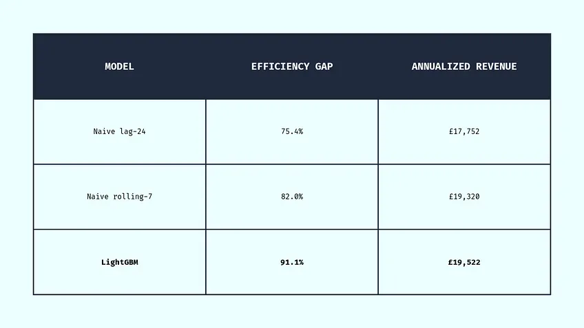
Because GB is an island grid with cross-border interconnectors, it’s a bit harder to get forecasts accurate. Every megawatt that flows through those interconnectors is a pre-scheduled commercial transaction, as opposed to an automatic response to a frequency imbalance the way continental AC interconnectors work. This means that GB’s prices respond more sharply to domestic supply and demand dynamics, with less buffer from neighboring supply.

The naive models struggled with this because they can’t distinguish between a January or June evening at the price levels, but with the ML model, the model would have had enough examples to learn those seasonal differences and it showed up in the inference results.

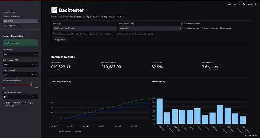
We also saw from the predicted P&L chart that January was the highest month, and revenue stayed moderate through spring and summer, and then dips as demand falls and solar flattens the intraday spread around July & August, then demand peaks back up going into the winter.

The GB model returns around £19.5k revenue against a £150k capital cost. Lower than Germany, but it did reveal that a battery operator would need to lean on frequency response and balancing markets alongside arbitrage to justify the capital.

Germany #

Germany produced the strongest results in this analysis, with the naive rolling-7 model outperforming LightGBM by 2.4%.

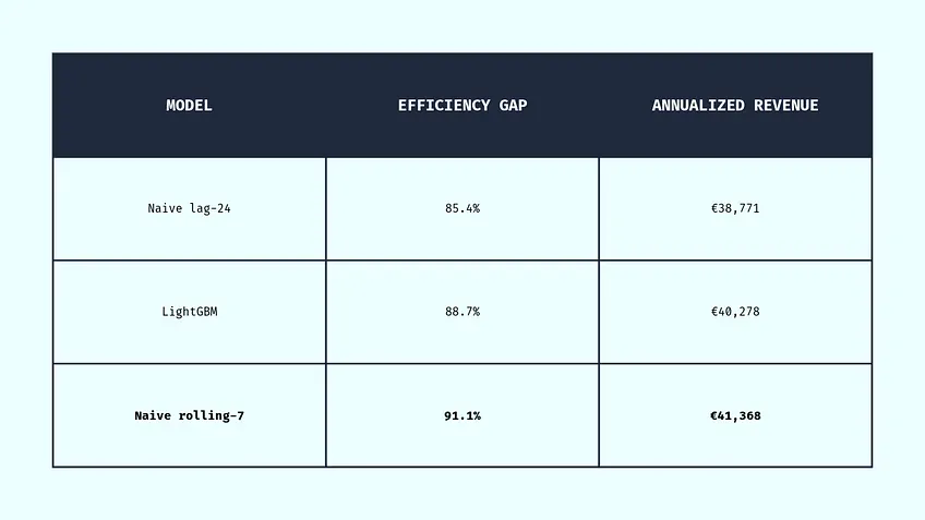
Germany is the most liquid electricity market in Europe, and its day-ahead price profile is stable and has a (mostly) repeatable price profile. That repetitive weekly structure is what the rolling-7 model can exploit. Because it averages the same hour across the previous seven days, it captures the weekly cycle without the added complexity of a learned model.

LightGBM landed in the middle at 88.7%. It learned the same structure, but because it’s working from a pooled model that uses multiple zones for its training set and has more parameters to fit, there was room to pick up patterns from the training data that don’t necessarily persist into 2025. Rolling-7 has no parameters so it can’t overfit.

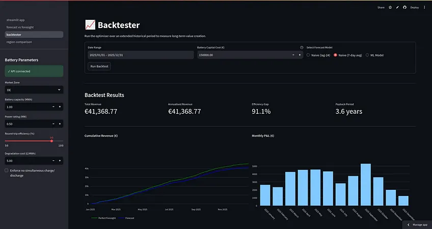
The predicted revenues were low in January and February meaning the market was relatively calm during the winter, then built up steadily through spring and summer, having a spike in October. The peak at around autumn is consistent with the pattern of German renewable generation falling as daylight shortens and gas and coal plants step in to meet demand. The evening peak ramp became sharper and more valuable to arbitrage.

A battery in this market, based on our ML model, would have earned roughly €41k against a €150k capital cost, and one of the most attractive results in this analysis.

Learnings & What I’m Doing Next #

When I first started building this, I’d expected the LightGBM model to consistently outperform the naive baselines— and it mostly did when I trained a new model for each zone initially. When I decided to pretrain because of Streamlit’s memory issues causing the training runs to fail on the deployed version, the quality of the model’s predictions fell because of more noise in the pooled model.

The GB model shined because I kept it separate due to how different the markets were, but it still only slightly outperformed the baselines.

Two things stood out to me while building this: first, pooled models trade market zone-specific fit for generalizability, and rolling-7 beat LightGBM in Germany precisely because it has no parameters to overfit with. Second, GB’s island grid structure made forecasting harder than continental markets, and the model trained only on GB data still only barely outperformed the seven-day average. Both of these pointed to the same learning; that better features matter more than a more complex model.

It had me wondering what features would make the models better still, and what added complexity would look like in a system that needed to update charging schedules across thousands of batteries daily.

For a grid-scale battery, the day-ahead market is only one of several revenue streams available. Real operators participate in the balancing, frequency response and capacity markets simultaneously, and understanding how to optimize across more of them, across distributed resources, is where I want to go next.

You can check out the tool here, and the Github repo here :)

Until next time!