I built an optimization model to figure out where batteries should go on a power grid.

Energy storage is becoming critical infrastructure as renewable energy integration grows. But because batteries are expensive and utilities have limited budgets, where you place storage on a grid matters enormously. Not just for profitability, but for grid reliability and how much renewable energy a grid system can actually use.

Heuristics like “put storage near the wind farms” or “near big cities” are intuitive, but they often miss a crucial point. The power grid is a network, and value emerges from how all pieces interact, not just from local conditions.

I built an optimization model to find the provably best storage location for a 24-bus power network under different demand and wind generation scenarios. The model considers generation costs, transmission constraints, battery physics, and competing priorities(keep the lights on cheap vs. use more renewables) simultaneously.

In this post, we’ll walk through:

• The optimization problem and how I modeled it
• Six scenarios that show how storage value changes with grid conditions
• Why some results were counter intuitive
• And what this means for real-world grid planning

Grid-Scale Storage Allocation #

Grid operators juggle three competing objectives every hour of every day:

1. Reliability: Keep the lights on(penalty for load-shedding/blackouts)
2. Economic efficiency: Minimize generation costs(use cheap baseload and avoid expensive peaker plants)
3. Environmental goals: Maximize renewable energy use( penalty for wasted wind)

You can’t really optimize for one without considering the others. Storing cheap coal power saves money but doesn’t help renewables, and putting storage near wind farms might help environmental goals but might miss reliability improvements from placing it near demand centers(nodes where energy is consumed by end-users).

Grid planners often use rules of thumb:

• Co-locate storage with renewables: captures excess wind, but ignores power flows through the transmission network
• Put storage at high demand buses: makes sense for reliability; might miss opportunities for temporal arbitrage elsewhere
• Spread evenly across the network: fair, but some buses might have 10x the value of others

These heuristics come from good intuitions, but can’t handle the full complexity. A power grid has hundreds of interacting constraints: generator ramp rates, transmission line capacities, battery charge/discharge limits, and power balance at every bus and every hour. These constraints make the number of possible storage allocations explode combinatorically.

And unlike a machine learning model, an optimization model ensures that Kirchhoff’s laws are never violated, whereas an ML model could hallucinate a physically impossible power flow. An optimization model:

• Finds the provably best solution given your objectives and assumptions
• Considers all constraints simultaneously (physics + economics + reliability)
• Reveals non-obvious interactions (like why a transmission hub with no local activity could turn out to be valuable)

The Problem I modeled #

Network topology: The network topology I used here is a 24-bus IEEE reliability test system where we have:

• 24 buses (nodes where power is generated, consumed, or transmitted)
• Each transmission line has a capacity limit (if power flow exceeds this, you get congestion)
• Power can’t teleport; it has to flow through the network following Kirchhoff’s laws

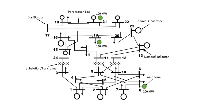
Our optimization question: Over a 24-hour period, which buses should get how many storage units to minimize total operating costs while maintaining reliability and maximizing renewable integration?

I formulated this as a Mixed-Integer Linear Program. In MILP, the objective function(the expression representing the goal to be optimized) and all constraints are linear, which means that we can use modern solvers to find globally optimal solutions. I’ll explain this in a bit, but I simplified some real-world complexities like the quadratic generator costs to keep the function linear, which is a reasonable trade-off for planning purposes.

The Function

Minimize:

Σ (Generator Cost × Output)

• £10,000/MWh × Load Shedding

• £50/MWh × Wind Curtailment

$$\text{OF} = \sum_{g,t} a_g(P_{g,t})^2 + b_g P_{g,t} + c_g + \sum_{i,t} \text{VOLL} \times \text{LS}_{i,t} + \text{VWC} \times P_{i,t}^{\text{pwc}}$$

Subject to the following constraints:

$$\sum_{g \in \Omega_i^G} P_{g,t} + \text{LS}_{i,t} + P_{i,t}^w - L_{i,t} - P_{i,t}^c + P_{i,t}^d = \sum_{j \in \Omega_i^L} P_{ij,t} : \lambda_{i,t} $$ $$P_{ij,t} = \frac{\delta_{i,t} - \delta_{j,t}}{X_{ij}}$$ $$P_{ij,t} = \frac{\delta_{i,t} - \delta_{j,t}}{X_{ij}}$$ $$-P_{ij}^{\max} \leq P_{ij,t} \leq P_{ij}^{\max}$$ $$P_g^{\min} \leq P_{g,t} \leq P_g^{\max}$$ $$P_{g,t} - P_{g,t-1} \leq \text{RU}_g$$ $$P_{g,t-1} - P_{g,t} \leq \text{RD}_g$$ $$0 \leq \text{LS}_{i,t} \leq L_{i,t}$$ $$P_{i,t}^c = w_{i,t} \Lambda_i^w - P_{i,t}^d$$ $$0 \leq P_{i,t}^w \leq w_{i,t} \Lambda_i^w$$ $$\text{SOC}_{i,t} = \text{SOC}_{i,t-1} + \left(P_{i,t}^c \eta_c - \frac{P_{i,t}^d}{\eta_d}\right) \Delta_t$$ $$P_{i,\min}^c \leq P_{i,t}^c \leq P_{i,\max}^c$$ $$P_{i,\min}^d \leq P_{i,t}^d \leq P_{i,\max}^d$$ $$\text{SOC}_{i,\min} \times N_i^{\text{ESS}} \leq \text{SOC}_{i,t} \leq \text{SOC}_{i,\max} \times N_i^{\text{ESS}}$$ $$\sum_i N_i^{\text{ESS}} \leq N_{\max}^{\text{ESS}}$$

Key Constraints:

• Power Balance: This is Kirchhoff’s current law: power in must equal power out at every node. If this isn’t satisfied, you get blackouts or voltage instability.

• DC Power Flow: This is a linear approximation of AC power flow. It captures transmission constraints and congestion without the full complexity of considering reactive power and voltage magnitude, which is good enough for planning studies like this.

• Generator Constraints: For our generators, many plants can’t produce less than a minimum stable output because they can’t turn off completely, and all can’t produce more than maximum capacity

• Transmission limits: Each transmission line has a thermal limit to avoid overheating. When lines hit their limits, you get congestion, and power from cheap generators in one region can’t flow to reach demand in another region. Storage on both sides of a congested line can arbitrage this difference.

• Energy Storage Physics:

  • State of charge: Energy stored in a given hour equals the energy from last hour, plus what you charged(with ~95% efficiency), minus discharge(with ~90% efficiency). Round-trip efficiency is about 85%, realistic for most lithium-ion batteries.
  • Capacity bounds: basically means we can’t store more than a battery’s capacity, and we also can’t charge in the negatives
  • Power bounds: This means we can’t charge or discharge faster than a battery’s power rating.
  • Cyclical constraint: A battery must return to its starting state at the end of the day. This is to prevent the battery from cheating by treating the battery as a one-time energy source, rather than a storage device that cycles daily.
  • Budget Constraints: We can’t place unlimited storage because units are expensive. In the original notebook, I worked with a maximum of 5 units per bus, and 15 units total across the grid, and for the final dashboard, I left the total units across the grid open to play with.

Building the dashboard #

I used Pyomo to build the optimization model, which is a solver-agnostic optimization package in Python. It lets you write constraints in algebraic notation that’s pretty close to how you’d write them mathematically, and translates your model into a standard format that most solvers can read.

For the solver I used GLPK(GNU Linear Programming Kit), which is an open-source solver that implements algorithms for MILP problems. For our problem size(pretty tiny) GLPK solves it in about 10-20 seconds on a laptop. Commercial solvers like Gurobi or CPLEX would be a lot faster, but GLPK is free and good enough for this.

Finally, I used Streamlit to go from notebook to a dashboard that allows users to play with demand and wind scenarios, adjust the storage budget, and unit capacity with sliders.

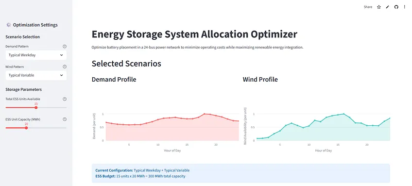
I also used Streamlit’s caching feature to save time running different scenarios, so if you run the same scenario twice, you see the cached results instantly instead of re-solving.

Scenarios #

When I started building this, I worked on only one demand-generation profile, which was a normally distributed series of values generated with NumPy.

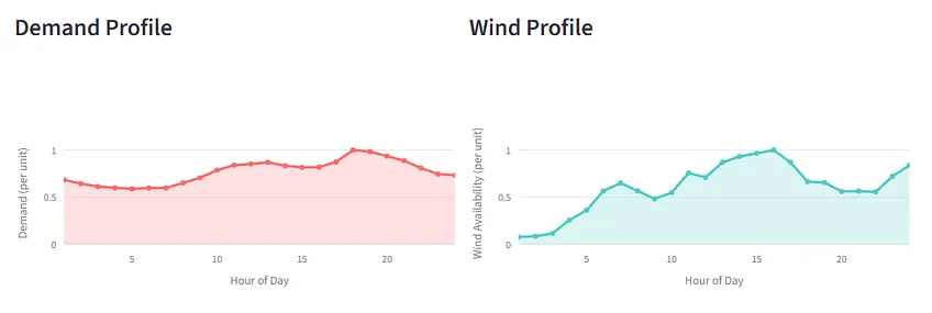
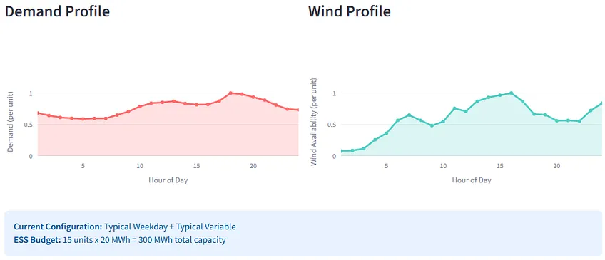
Then I generated three more demand and wind profiles based on realistic patterns, which gives us 16 possible combinations to explore, making the dashboard more interactive.

Result Analysis #

On the dashboard, you can play with a total of 16 different combinations of both profiles, and tweak the number of battery allocation and the unit capacity of the batteries, but for brevity, I’ll be analyzing only 6 of them here.

SCENARIO 1: BASELINE (Typical Weekday + Typical Variable Wind) #

The Setup:

To understand the results of the optimization better, I generated a table with the bus allocations each time a scenario is run.

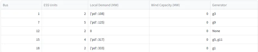
Here, a cool thing is that on Bus 12, we have two storage units allocated despite the bus being the only one with zero demand and generation. This likely means that the bus is a transmission hub in the grid, and the solver recognizes and places batteries there to manage flow congestion between the other buses.

Another thing you’ll notice(and across most of the results) is that the wind curtailment cost is tiny. Because of the ratio of penalties for the VOLL:VOLW is essentially 200:1, the model will always prioritize keeping the lights on cheaply over saving greener energy. We could force the model to use more wind by increasing the VOLW, but that’s for a future version.

Total Costs: £401,295 [Generation(£399,480) + Wind Curtailment(£1,815 for 36.3 MWh)]

SCENARIO 2: Winter Peak + Windy Day #

The Setup:

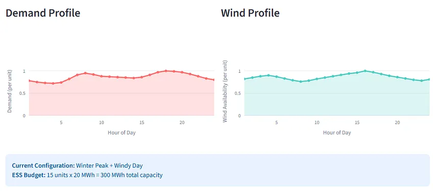
The model placed three units at Bus 21 in this scenario because in this scenario, we have much higher wind output, so the model co-located some units to that bus to absorb the energy and avoid curtailment costs despite it being a windy day. The battery then acts as a buffer to smooth out the wind supply through the grid. Buses 5 and 9 got 5 units each, acting as transmission hubs to balance the load across the grid.

Total Costs: £413,963 [Only generation costs]

SCENARIO 3: Typical Weekday + Night Wind #

The Setup:

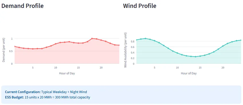
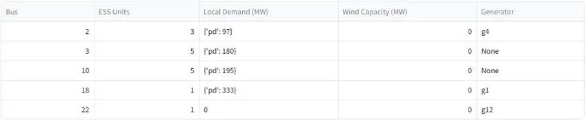
The model placed 5 units at Bus 3 despite having no generators to avoid congestion during peak hours of the weekday. Bus 3 is a substation(as indicated in the diagram), and also serves as a crucial transmission hub, like bus 10, which also got allocated 5 units despite no generators. Buses 2, 18, and 22 got 3, 1, and 1 units respectively, suggesting that they were allocated to serve as buffers to avoid turning on peaker plants. Interestingly, no units were allocated to any buses with wind farms in this scenario.

Total Costs: £412,400 [Only generation costs]

SCENARIO 4: Weekend Low + Calm Day #

The Setup:

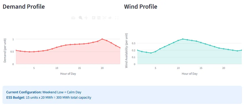
This scenario proves that the model works even when wind generation is scarce. Here, wind profile is low, and yet the model was still able to deploy full storage.

Since there is no excess wind to save, the batteries were deployed at bus 23 which hosts two generators, which means they are likely energy arbitrage batteries in this case. The model can see that running cheap thermal generators at a steady output to store energy during the low demand afternoon, and releasing it during the peak hours of the evening to avoid turning on expensive peaker plants and increase generation costs.

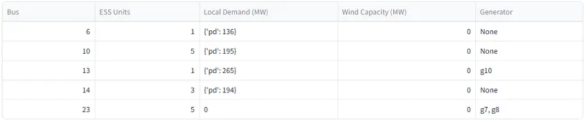
Total Costs: £411,312 [Only generation costs]

SCENARIO 5: Summer Peak + Night Wind #

The Setup:

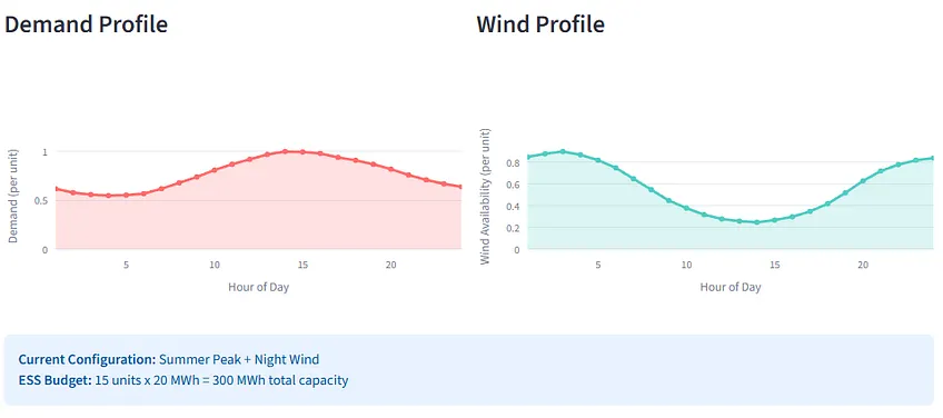
In this scenario, the model worked a lot harder to shift energy across time periods. Unlike the winter/windy scenario, this scenario makes the model spread small units all over our network to try to fight local congestion. The idea is to inject power locally at multiple load centers during the afternoon peak period to avoid overloading transmission lines.

The main cause of this is because supply and demand were opposites here(wind at night, demand in the day), and the model moved away from clustering batteries and distributed them next to load centers to dispatch energy during the peak.

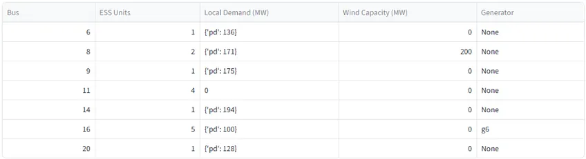
Total Costs: £424,169 [Only generation costs]

SCENARIO 6: Winter Peak + Calm Day #

The Setup:

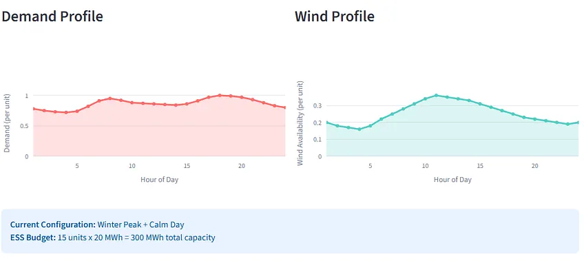
These might just be the worst conditions I had(read: most expensive). Other scenarios generally cost around low-mid 400k, but here we got a generation cost of 510,095. The storage units were also more spread through the grid than before, with only buses 6 and 23 receiving 5 units each. Bus 6 likely serves as a transmission hub in addition to its own demand as shown in the diagram, while bus 23 could be an energy arbitrage opportunity to meet the energy demands by running the two thermal generators and dispatching it over the grid throughout the day. This bus has no demand of its own, but plays a key role in balancing the load through the grid, while bus 19 is allocated 2 units to absorb wind energy and avoid curtailment.

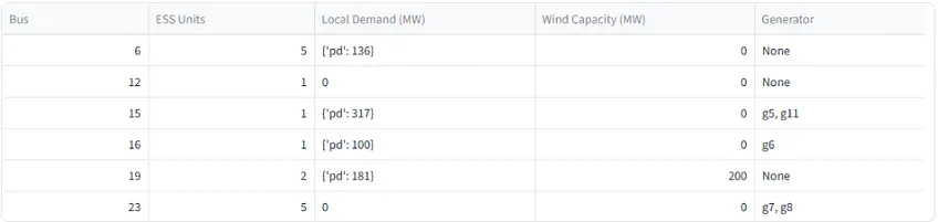
Total Costs: £510,095 [Only generation costs]

SUMMARY #

The table below summarizes allocation patterns across all six scenarios:

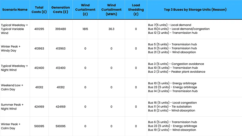
PATTERNS ACROSS SCENARIOS #

After running all the scenarios, there were patterns that stuck out to me across the different conditions:

1. Network topology would consistently dominate local conditions: Something I noticed consistently was that buses that acted as transmission hubs got allocated storage despite having no local demand, thermal power generation, or wind farms. This is because when transmission lines get congested(which happens often under high wind or high demand scenarios), having storage at such hubs help move power between regions more efficiently. This kind of insight often can’t be gotten with ML or heuristics, because the value of models like this emerge from network effects, not local activity. You can’t plan grid infrastructure just by looking at buses in isolation; it’s often more valuable to model the full network and transmission constraints

2. The VOLL/VOLW ratio drives trade-offs: In the optimization model, I set: VOLL(Value of Lost Load): £10,000/MWh and our VOLW(Value of Lost Wind): £50/MWh. This 200:1 ratio means the model will do almost anything to avoid blackouts, but is mostly alright with wasting renewable energy. This reflects utility priorities in most grids today: reliability first renewables second. I ran an experiment increasing the wind curtailment penalty to £200/MWh and kept the VOLL at £10,000/MWh. It wasn’t enough to force the model to allocate storage to the wind farm, but the curtailment cost did increase from £1,815 to £7,259 for the same MWh. However, in the winter peak + windy day scenario, the model allocated 5 units to the wind farm at bus 19(unlike the 3 at bus 21 before) and spread out the remaining units across a transmission hub(bus 22) and buses 2(generator + local demand) and 9(only local demand). The shift from bus 21 to bus 19 is likely because bus 21 was no longer optimal due to the increased cost of curtailment and bus 19 having both demand and a wind farm, and bus 21 having no demand at all. Bus 21 was likely able to move the power generated across the grid to other demand buses and storage units since there were no curtailment costs here.

3. Storage complements transmission: In several scenarios, storage went to buses that were transmission-constrained, not generation or even demand-constrained. This suggests that storage can partly compensate for a transmission bottleneck, but it’s not a replacement for building adequate transmission infrastructure. They’re complementary investments, which means that grid planning should be asking “how much of each should we build, and where?” A co-optimization model that includes both transmission expansion and storage allocation as decision variables could be even more powerful.

4. Storage value is highest under temporal mismatch: Storage is fundamentally about time-shifting. When supply and demand are naturally aligned(windy when demand is high, for example), storage adds less value. When they’re mismatched however(windy night, high-demand day, for example) storage is a lot more critical. The same battery could have 3x the value in one grid versus another depending on the demand/supply patterns.

Limitations #

Building this model taught me loads, but I think it’s important to talk about some of the limitations it currently has:

1. DC power flow approximation: without this, we wouldn’t have an MILP problem, we’d have a non-linear objective function that’s harder to handle and only finds locally optimal solutions. A DC approximation is a linearized model of power flow that ignores reactive power(i.e. the imaginary/bidirectional component of AC power), voltage magnitude constraints, and resistive losses in transmission lines. They matter way more for operational decisions(like voltage stability, which grid operators care a lot about). For planning studies like this where we’re asking “where should storage go”, DC power flow captures the main effects: transmission limits and congestion.
2. Perfect foresight: I’m also assuming we know demand and wind generation values perfectly 24 hours in advance. In reality, forecasts have (sometimes significant) errors. A wind forecast might predict 70% capacity but the actual output is 50% or 85%. Demand forecasts can also be way off during heatwaves or cold snaps. This uncertainty changes optimal decisions. If you’re not entirely sure you’ll need storage capacity tomorrow, a grid operator might want to keep batteries partially charged(called hedging), whereas perfect foresight lets you drain them completely.
3. Simplified generator costs: My model uses linear cost functions, but real generators have quadratic costs that increase with output in addition to startup/shutdown costs, and minimum up/down times (i.e, can’t cycle on or off hourly). This is called a unit commitment problem, and it’s essentially still MILP but with more binary variables and constraints.

Quick note: Startup/shutdown costs are not the same as ramp-up/ramp-down costs. The former are the fixed(step-wise, for the fancy) costs incurred to turn a generator on/off, and this could include fuel consumed during ignition, maintenance, and labor. The latter are more variable costs associated with changing the output level(MW) .

Final Note: #

With more coal plants retiring, electric vehicle adoption scaling up, and renewable energy. Globally, renewable energy capacity has been projected to increase almost 4600GW between 2025 and 2030, which is double the deployment of 2019-2024. Energy storage is a critical enabling technology to increase the penetration of renewables, but utilities can’t afford to build storage everywhere. This is why planning studies like this are important in order to get the most value out of investments made in grid storage.

We’re adding renewables faster than we’re adding storage/transmission, and optimization models can help us understand where new additions to the grid would be most valuable

The model is simplified, but the approach could scale to larger networks and more complex decisions like combining storage, transmission and generation planning.

What’s Next? #

The current optimization model takes 10-20 second to solve, which is fine for planning, but too slow for real-time dispatch. In my next project, I’m going to explore optimization across distributed energy resources for real-time grid balancing. The goal is to learn more about forecasting models and potentially quantify whether (and at what cost) home energy resources can provide grid services as effectively as peaker plants.

---

Have a look around the dashboard and play with some of the scenarios here:

https://essallocator.streamlit.app/

Open to questions and feedback!